The tunes in the Ottawa Slow Jam collection are divided into several volumes and appear to be arranged so that consecutive tunes can be played in sets. As a result about 95 tunes are duplicates since they were part of different sets. For purposes of extracting statistical data, I have attempted to remove most of the duplicates. You can download the collection that I used here.
With many exceptions, Celtic music follows the following structure. A tune is divided into an A and B part each of which is eight bars long. The tunes can be grouped by their rhythm: jigs, reels, hornpipes, waltzes, etc. The different forms were divided as follows.
| reel | slide | jig | double jig | slip jig | hornpipe | polka | waltz | march |
| 189 | 11 | 153 | 6 | 19 | 47 | 39 | 54 | 22 |
|---|
There were numerous other forms such as dances, songs, airs, lamentations and others that are part of the collection but not enumerated in this table.
The music is written in various modes such as major, minor and dorian. The distribution shown below is not exact since a few of the tunes are a combination of two or more modes -- for example major and relative minor.
| A | Ador | Amin | Amix | Bdor | Bmin | Bphr | C | D | Ddor | Dmin | Dmix | E | Edor | Emin | G | Gm |
| 45 | 39 | 13 | 19 | 1 | 11 | 1 | 6 | 198 | 2 | 2 | 34 | 2 | 25 | 23 | 189 | 2 |
For those not familiar with modes and scales, an octave is divided into 12 notes. If all 12 notes are used, the scale is called chromatic. This corresponds to using all the black and white keys on a piano. Western folk music generally uses a subset of 7 notes from the chromatic scale. For example the C major scale consists of just the white notes on the piano. If C is the first note of the scale and the tonal centre of the piece, the mode of the scale is called major or less commonly ionian. Assuming there are are no flats and sharps in the scale, the dorian mode begins the scale with the next note D, the mixolydian scale begins with G, and the minor (aeolian) scale begins with A.
Furthermore some of the tunes use only 5 (pentatonic) or 6 (hexatonic) notes in the scale. If all seven notes are used, which occurs in the majority of cases, the scale is called heptatonic.
It is not obvious from the sequence of sharps or flats in the key signature whether the mode is major, dorian, minor, etc. In particular the Celtic Slow Jam collection does not label the music with these different modes. I have tried to do my own labeling based on the tonal centre and the final note of the tune.
This note describes two methods of analyzing a collection of abc tunes: 1) identifying common music sequences and 2) matching pitch histograms. To illustrate, consider the following pair of tunes.
Common sequences are highlighted in red. When you play the corresponding MIDI files, the two tunes sound somewhat similar. The Lilting Banshee and Three Little Drummers
Now consider the following pair.
The first tune is a double jig and the other is a hornpipe. Though there are almost no common sequences in the two tunes, they still sound somewhat similar. Tobin's Favorite and Byrne's Hornpipe
If one compares the pitch distributions of the two tunes they are almost identical implying that they share a common tonality.
 |
 |
| Tobin's Favorite | Byrne's Hornpipe |
|---|
Numerous studies have used histograms of the pitch intervals between adjacent notes. Though I found this approach to be somewhat successful in identifying duplicates in our database, the method did not seem to identify similar sounding tunes.
The rest of this note is divided into two sections. The next section deals with the subject of common bars and common note sequences. The last section deals with histogram matching.
Analysis of the collection detected only a few instances where the same sequence of bars occurs. The following example Sporting Pitchfork and Cook in the Kitchen is one such instance where the first tune ends with a sequence of bars found in the second tune.
A few other pairs of tunes had three or more bars in common. In some cases they were even consecutive like the second sections of "The Cow that Ate the Blanket" and "The Pet of Pipers".
| Mist on the Mountain | Trip to Bantry |
| Gold Ring | Hartigan's Fancy |
| Gold Ring | Kilfinane |
| The Cow that Ate the Blanket | The Pet of Pipers |
| Hill on the Road | Blooming Meadows |
| Buckley's Fancy | Reavy's |
Though they sound and look very similar, only a few musical bars match exactly. The bars which do not match have trivial differences and exposes some of the limitations of our matching scheme. There is also question of whether they are both the same tune with different names and minor variations. Other pairs belonging to this class are
| Out on the Ocean | Portroe's Jig |
| Kerry Slide | Kathleen Hehir's Slide |
| Croppies' March | Bank of Inverness. |
In general we did not find many examples of borrowed musical measures in this collection. Waltzes and other music in 3/4 time tended to have two to three notes in a musical measure which leads to many nonsignificant matches.
Frequently one finds an isolated measure that occurs in another tune, but based on its context it seems that this was an accidental effect. The measure that was repeated is often an arpeggio or an ascending or descending sequence. A function was written which which scans the entire collection of tunes using each tune as a template for comparing it with the other tunes. Pairs of tunes containing common bars were reported.
Various matching strategies were investigated. In absolute mode, the sequence of matching notes must occur in the same relative positions in the musical scale. Thus CDE in the scale of Cmaj would match GAB in the scale of Gmaj. However CDE in Cmaj will not match GAB in Cmaj. The idea of absolute mode is that the context of melodic contour is also important. On the other hand, in contour mode only the shape of the musical contour is important. Thus CDE would match GAB in the key of C major. Contour mode is less restrictive and catches more matches. Other strategies ignored the rhythmic information or allowed one or two insertion, deletion or substitution errors.
Many matches were reported by the function. Here is a an excerpt from a short run.
grouper output at Thu Dec 19 06:20:01 EST 2013
for C:/Users/User/abc/tcl/OSJ_all_nodup.abc
33 tunes matched out of 40
the 33 tunes had a total of 695 bars
average number of tunes linked to matched tune = 10.09
elapsed time = 2
  for 1  The Kesh Jig (17 bars)
2  Blackthorne Stick (2-1 bars)
5  The Mug of Brown Ale (1-1 bars)
6  Mist on the Mountain (Jig) (1-1 bars)
11  Saddle the Pony (2-1 bars)
16  The Cow that Ate the Blanket (1-1 bars)
20  The Frost is all Over (1-1 bars)
27  The Top of the Cork Road (Father O'Flynn) (2-1 bars)
169  Fainne Oir Ort (2-2 bars)
etc…
The number of bars matching bars in the compared tune m and the number of matching bars in the template n is indicated as the pair "(m-n bars)". In order to reduce the amount of output, the algorithm was suppressed output if fewer than n bars in the template matched. The scan was repeated on the set of 616 tunes with various run time parameters. The table below shows some typical results.
| Conditions | bars | matches | connectivity |
|---|---|---|---|
| exact absolute | 1 | 455 | 7.8 |
| 2 | 187 | 3.2 | |
| 3 | 60 | 2.2 | |
| 4 | 22 | 1.3 | |
| 5 | 4 | 1.0 | |
| 6 | 1 | 1.0 | |
| exact contour | 1 | 495 | 11.7 |
| 2 | 238 | 3.9 | |
| 3 | 90 | 2.4 | |
| 4 | 23 | 2.1 | |
| 5 | 11 | 1.6 | |
| 6 | 4 | 1.0 |
The second column bars indicates the minimum number of bars in the template that must be matched in order for a tune to be reported as a match. The third column matches indicates the number of tunes in the collection which had matches. The last column connectivity indicates the average number of tunes that were matched to the template.
As expected, more matches were found using the contour matching criterion. Most of the matches were false positives, in the sense the existence of a common bar in the pair seemed to be accidental and otherwise the two tunes had little in common. Pairs of tunes that had many matching bars were more likely to sound similar.
The number of template tunes which matched other tunes appears to fall off geometrically as the threshold number of bars (in the second column) increases. This suggests that the probability of the occurrence of matching bars is independent of the number of matching bars detected so far. This independence suggests that most of these matches are accidental. Nevertheless if two tunes have many bars in common, they sound somewhat similar.
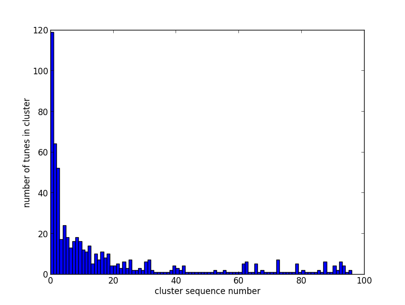
About 120 tunes out of the 616 tunes in the database did not match any other tune. Those tunes did not have any striking characteristics but tended to have a large number of notes in almost every bar.
The pitch histogram indicates the number of times each of the 12 notes in an octave is used in a particular tune. In this study, the frequency of occurrence of the notes was also weighted by the duration of the note (half note, quarter note, eighth note etc). The histogram was normalized to probabilities so that it could be compared with other distributions.
One can expect that the histogram would be sensitive to the key signature of the tune. Not all of the 12 notes in an octave are used for a particular key, and they would be missing from the histogram. It will be demonstrated that the pitch histogram is frequently closely related to the tonality of the piece.
The pitch histogram may be viewed as a 12 dimensional feature vector or a descriptor of the tune. If this data was one or two dimensional, it would be fairly easy to visualize its structure. For example, by producing a correlogram one can see the distribution of data points where each data point is a feature vector. Beyond two dimensions, one must compute various two dimensional projections in order to visualize the distribution. For higher dimensional data, one must rely on statistical computational algorithms to reveal the characteristics of the data. These techniques fall into the subject called 'pattern recognition' or 'data mining'.
Music tonality deals with the musical scale which forms the basis of the tune. Most western listeners are familiar with the major and minor scales; however, there are many other scales or modes used in traditional music. For example, see A Comparative Study of Indian and Western Music Forms (Agarwal and Karnick)which was presented at ISMIR 2013 conference. With regard to Celtic music, much of the music is also in the Dorian and Mixolydian modes besides the familiar major and minor modes. When one includes the gapped scales, pentatonic and hexatonic, (see Scales and Modes in Scottish Traditional Music by Jack Campin), there are many more scales.
In this collection, the key signatures had zero to three sharps corresponding to the keys of C, G, D, and A major. Though the majority of the tunes are in the major mode, about a quarter of these tunes were in one of the other Celtic modes such as dorian, mixolydian and minor (aeolian). About 25 tunes are based on a pentatonic scale and about 150 tunes use a hexatonic scale.
We shall now illustrate the application of pitch histograms, with the following plot Scatter the Mud.
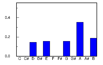
Observe that only five pitches occur in this tune. Though the music is in the key of A dorian, which shares the same key signature as G major, the notes C and F# are both missing. This is an example of a Dorian pentatonic mode. The tonal center, key of A is the most predominant pitch and the tune ends with A. Though the predominant pitch in the histogram is often the tonal centre, there are some exceptions. For example "Harvest Home" is in the key of D, but A is the predominant pitch.
When we compare the pitch histogram of "Scatter the Mud" with other tunes in the collection, we discover that there are at least 3 other tunes in the same key that exhibit the same pitch histogram. The tunes Brenda Stubbert's, Dan O'Keefe's, and Three Little Drummers are also pentatonic A dorian, and their histograms match the tune "Scatter the Mud". Though the melodies are different, there seem to be some similarities in the mood. In particular it seems that "Three Little Drummers" seems to be somewhat similar to "Scatter the Mud".
If we continue searching for pitch histogram matches using other tunes as the template, we find quite a few matches. For example, see the tables below.
| Title | C | C# | D | D# | E | F | F# | G | G# | A | A# | B |
|---|---|---|---|---|---|---|---|---|---|---|---|---|
| The Lady on the Island | 0.0 | 0.0 | 0.19 | 0.0 | 0.20 | 0.0 | 0.21 | 0.03 | 0.0 | 0.22 | 0.0 | 0.15 |
| Jenny Dang the Weaver | 0.0 | 0.0 | 0.16 | 0.0 | 0.20 | 0.0 | 0.23 | 0.04 | 0.0 | 0.24 | 0.0 | 0.12 |
| The Maid Behind the Bar | 0.0 | 0.02 | 0.18 | 0.0 | 0.15 | 0.0 | 0.22 | 0.03 | 0.0 | 0.22 | 0.0 | 0.18 |
This suggests that the pitch histograms may not be random but tend to cluster in groups. It would be informative if we could identify these groups using some computational procedure.
In this note we applied the kmeans mean-shift algorithm which is one of the six unsupervised classification algorithms in the scikit-learn. The clustering page on that web site illustrates the characteristics of these six algorithm on different sets of two dimensional data. One of the characteristics of the kmeans mean-shift algorithm is that it does not require you to assume a certain number of clusters in the data. Instead the algorithm returns the number of clusters and converges to the cluster centers. However, the algorithm does require you to provide the size of a search window which is called 'bandwidth'. The number of clusters that are returned depends on this measure. The algorithm is somewhat slower than the regular kmeans algorithm when the size of the data set and dimensionality is high; but in this situation the computation time was just a few seconds.
A description of how to use the scikit-learn library is given in the appendix of this note.
Each of the tunes in our collection is associated with one pitch histogram vector. When the mean_shift algorithm was applied to this collection, it assigned the pitch histogram vectors to one of 96 clusters. The clusters are not of equal size and most of the tunes were assigned to the first 20 or so clusters. Some clusters contained only one pitch histogram vector and they could be viewed as 'outliers'. The plot below shows how the tunes were distributed among the 96 clusters.
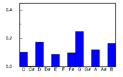
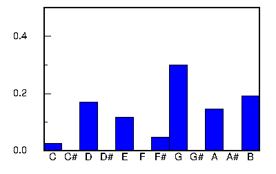
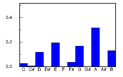
It is instructive to look at the cluster centres returned by the algorithm. Each row of the table represents the average pitch histogram for one of the 10 clusters. The size column is the number of tunes (or pitch histograms) that were matched to this cluster by the algorithm. The variance column indicates the mean square variation of the sample pitch histograms about the centroid. If you divide this by 12 and take the square root, this would be the standard deviation of each histogram value about the mean (assuming the clusters are spherical in the 12 dimensional feature space).
| Number | Size | Variance | C | C# | D | D# | E | F | F# | G | G# | A | A# | B |
|---|---|---|---|---|---|---|---|---|---|---|---|---|---|---|
| 0 | 119 | 0.0103 | 0.003 | 0.053 | 0.244 | 0.000 | 0.144 | 0.000 | 0.199 | 0.102 | 0.001 | 0.177 | 0.000 | 0.076 |
| 1 | 64 | 0.0102 | 0.102 | 0.004 | 0.173 | 0.001 | 0.087 | 0.000 | 0.099 | 0.248 | 0.001 | 0.120 | 0.000 | 0.166 |
| 2 | 52 | 0.0103 | 0.027 | 0.001 | 0.170 | 0.000 | 0.117 | 0.000 | 0.047 | 0.301 | 0.000 | 0.147 | 0.000 | 0.191 |
| 3 | 17 | 0.0075 | 0.027 | 0.008 | 0.118 | 0.000 | 0.195 | 0.001 | 0.036 | 0.168 | 0.000 | 0.316 | 0.000 | 0.131 |
| 4 | 24 | 0.0082 | 0.020 | 0.008 | 0.127 | 0.001 | 0.222 | 0.000 | 0.134 | 0.225 | 0.001 | 0.120 | 0.000 | 0.142 |
| 5 | 18 | 0.0072 | 0.114 | 0.005 | 0.122 | 0.000 | 0.167 | 0.003 | 0.034 | 0.172 | 0.002 | 0.282 | 0.000 | 0.100 |
| 6 | 13 | 0.0065 | 0.010 | 0.014 | 0.138 | 0.001 | 0.297 | 0.000 | 0.151 | 0.143 | 0.000 | 0.107 | 0.000 | 0.139 |
| 7 | 16 | 0.0079 | 0.000 | 0.168 | 0.081 | 0.000 | 0.190 | 0.002 | 0.130 | 0.003 | 0.043 | 0.273 | 0.000 | 0.111 |
| 8 | 18 | 0.0097 | 0.030 | 0.002 | 0.113 | 0.000 | 0.140 | 0.000 | 0.051 | 0.272 | 0.000 | 0.231 | 0.000 | 0.160 |
| 9 | 16 | 0.0079 | 0.094 | 0.022 | 0.237 | 0.000 | 0.123 | 0.004 | 0.167 | 0.138 | 0.000 | 0.174 | 0.000 | 0.040 |
Tunes that fit into a specific cluster generally have a common tonality. Cluster 0 consists of mainly tunes in the key of D major. Clusters 1 and 2 shown below are both in the key of G major, but the tunes in cluster 2 have a pentatonic tendency. Cluster 3 tunes are mainly in the key of A dorian or A minor.
The tables below list the first 10 tunes captured by matching the cluster pitch histogram centroid (shown in the graph on the right or in the above table). The degree of the match is given by the correlation coefficient which varies between +1.0 and -1.0. A value of 1.0 indicates that the tune's pitch histogram matches the centroid perfectly. A value of 0.0 indicates no correlation, and negative values indicate an inverse correlation.
There was no consistency between the correlation coefficient and the degree of similarity. In many cases a high correlation coefficient identifies tunes which sound similar; however, there were also matches that sounded different even though they shared the same tonality.
Outliers such as "Old Hag You Have Killed Me", "Pach Pi" seemed somewhat different. On the other hand, sometunes appeared as outliers merely because they were in a key which was not common for this collection (eg. D minor).
In summary, histogram matching provided another approach for separating tunes into groups and were found to yield a finer distinction than just the key signature.
|
 |
|
 |
|
 |
Some other collections such as the Eric Foxeley's Music Database which is also available in abc format on my web page were more varied and did not match our collection as well. Nevertheless there were some very nice jigs that I would like to include. The same comment also applied to John Chamber's collection of Irish Music. There are many music examples that I could add to this note; however, this web page is already getting bloated with MIDI files.
ipython
import numpy as np
from sklearn import cluster
a = np.loadtxt("OSJ_all_nodup.txt")
b = cluster.mean_shift(a,0.1)
np.savetxt("meancentroids.txt",b[0],fmt='%6.3f',delimiter='\t')
np.savetxt("assignments.txt",b[1],fmt='%5d')
c = np.histogram(b[1],96)
print(c)
print("finished")
The first line starts the ipython interpreter which is basically a Python interpreter with added features. The next two lines tell the interpreter to load libraries that will be used below. Numpy is a separate package which handles data in the form of "arrays" very efficiently and is used by the scikit package.
The pitch histograms of the collection of tunes were copied into a file called OSJ_all_nodup.txt. Each line contains one histogram corresponding to an individual tune and the 12 values of the histogram are separated by tabs. The file is loaded into a numpy array called a using the library function np.loadtxt(). The data in a is clustered by the mean-shift algorithm using a bandwidth value of 0.1. The results are stored in two arrays b[o] and b[1] and saved to separate files, meancentroids.txt and assignments.txt for further analysis. The latter file assignments.txt indicates the cluster assignments of each pitch histogram in a. The function np.histogram computes the histogram of the cluster assignments and saves it in the c array.